Intelligent Go Player
By Peihan Gao & Yiming Yan
Demonstration Video
Introduction
The game of Go, which originates from East Asia, is an abstract strategy game with a considerably long history. Go is complete information and zero-sum game, where two players respectively place the black and white pieces on a square board by turn for the purpose of finally occupying the larger territory. As the industry of artificial intelligence(AI) flourishes, the game of Go has been re-valued as a landmark problem during the process of exploring the unlimited potential of AI. In 2016, the AlphaGo Lee defeated the legendary professional Go player Lee Sedol (9 Dan) with a result of four to one. In 2017, the improved version AlphaGo Master victoried over the world number one professional player Jie Ke (9 Dan) in all three games. Soon later, the AlphaGo Zero, which was completely trained using reinforce learning without any human game records, defeated the AlphaGo Lee and AlphaGo Master in 100 : 0 and 89: 11 respectively [1]. These shocking and epoch-making achievements not only radically changed the way that human players hone their Go skills (It has been very common for both amateur and professional Go players to leverage Go AI to analyze their game record, which is quite hard to imagine before.), but also demonstrated that AI has the ability to independently explore complicated and abstract fields.
Project Objective
A powerful and lightweight Go analyzer, trained by a GPU device and running on a Raspberry Pi 3B+, has been implemented in this project. In detail, the core algorithm is the re-accomplishment based on the theories mentioned in the paper of “AlphaGo Zero”. Furthermore, a graphic user interface (GUI), displaying the analysis results of the core algorithm, has been developed and run on a Raspberry Pi.
Commercial Prospect
The opinion held by people about the AI Go program were sharply reversed after Lee Sedol lost to AlphaGo Lee. A revolution, which radically changed the way that both the amateur and professional players hone their Go skills, has happened. According to the statistics [4], there are currently 46 million Go players, which form a huge market, all over the world. Thus, a lightweight and highly intelligent Go analyzer, which can even run on a personal computer, will be saleable.
Rules of Go
There are many versions of the rules for the game of Go. Generally, the Chinese and Japanese rules are most popular among human players while the Tromp-Taylor rule is in wide use for AI players. In terms of the basic definition, these rules are completely identical. The main differences for them can be summarized as the suicide, territory calculation, compensation, and repeated grid coloring, all of which will be explained later [2].
Liberty
As a basic term of the game of Go, the “liberty” stands for the concept of “health points (HP)” owned by one piece or many connected pieces with the same color. For example, the black piece in Fig.2 has the liberty of four, marked by crosses, while the two pieces in Fig.3 have the liberty of six.
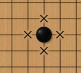
Fig. 2 Liberty of Four
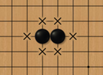
Fig.3 Liberty of Six
Take
If one piece or many connected pieces with the same color lose their liberty (liberty of zero), they will be taken (removed) from the game board. For instance, the black piece(see Fig.4) has only one liberty left. If it is currently the turn of the white player to move, the white player can choose to place the piece at the bottom of that black piece and take (remove) it from the game board (see Fig.5).
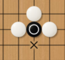
Fig. 4 Liberty of One
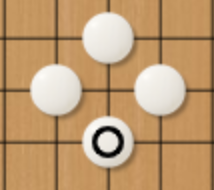
Fig.5 Take a Piece
Suicide
The position marked with a cross is obviously not a wise move for a white piece. That is because if the white player places the piece there, no black piece will be taken and the white piece will have no liberty. Thus, it is identical to suicide. The rules for human players ban a move like that. In terms of the Tromp-Taylor rule, although suicide is allowed, it will not bring any benefit for the player who makes a move of suicide. Additionally, if a move can take the pieces of the opponent, it will take the pieces of the opponent despite the fact that it initially has the liberty of zero (see Fig. 7 & 8).
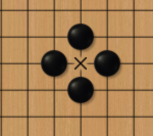
Fig.6 Suicide
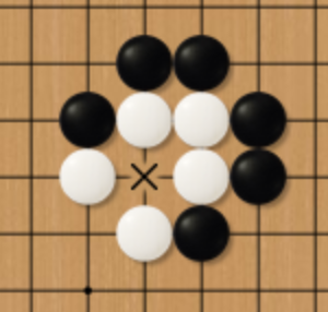
Fig.7 Special Situation
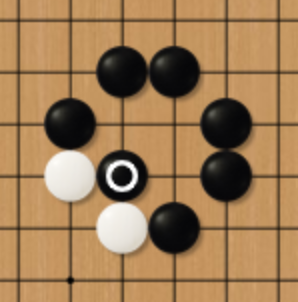
Fig.8 Take Pieces
Make True Eyes
As is shown in Fig.9 & 10, there are two “holes” surrounded by the black pieces. Both of them are called “eye”. There is no way for the opponent to take your pieces if you have two true eyes at the same time. That is because any attempt for you opponent to take your pieces will cause the suicide first. Thus, connected pieces with more than two true eyes will absolutely survive besides that you fill your own eyes (That will be obviously an unwise move). Additionally, the size and shape of the eyes (holes) can vary, only if there are at least two independent eyes (holes).
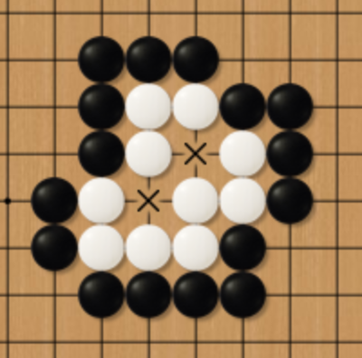
Fig.9 True eyes
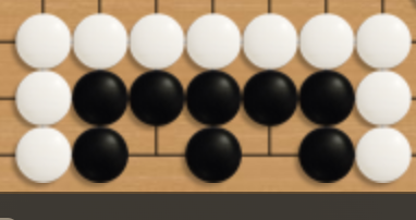
Fig.10 True eyes at the edge of the Game Board
Fake Eyes
There is also the concept of fake eyes, which is opposite to the true eyes. As is shown in Fig.11, the upper eye (hole) of the black piece is an example of the fake eye. The black pieces die anyway because the white player can gradually take all of the black pieces in two moves.
A similar situation also happens in Fig.12, the black pieces own a territory, whose shape is the same as the butcher’s knife. Although the black pieces still have the liberty of four, they will finally die because there is no way for the black pieces to make two true eyes without the help of the white player (That is definitely impossible).
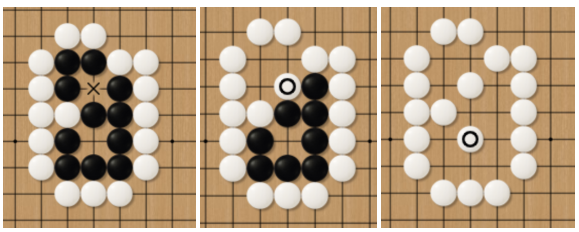
Fig.11 Fake Eyes
Fig.12 Butcher’s Knife
Seki
The term “Seki” describes an impasse that both sides cannot make two true eyes and both sides cannot take the pieces of the opponent (See Fig.13). In such a situation, the player who attempts to take the pieces from the opponent will be first taken by the opponent. In Fig.14, the white player attempts to take the black pieces. However, the white pieces die first. A similar situation is also demonstrated in Fig.15 for the black player.
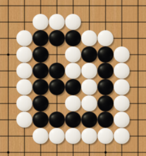
Fig.13 Seki (Impasse)
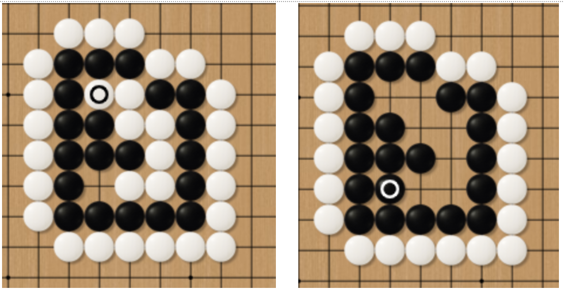
Fig.14 Unwise Attempt for White Players
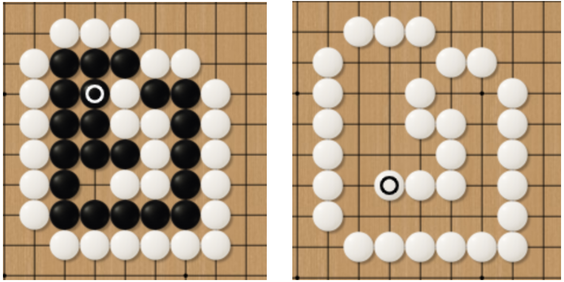
Fig.15 Unwise Attempt for Black Players
Territory Evaluation
The final winner will be generally determined by the comparison of the total territories occupied by two players. Before the final counting, all dead pieces should be taken from the game board. If there is an objection to the state (death or survival), two players should keep moving until the pieces are taken (death) or make at least true eyes (survival). Usually, human players will not raise an objection to the state of pieces in Fig.16 although the black pieces have only one giant eye now. That is because the black pieces can easily make two true eyes even the white player moves first.
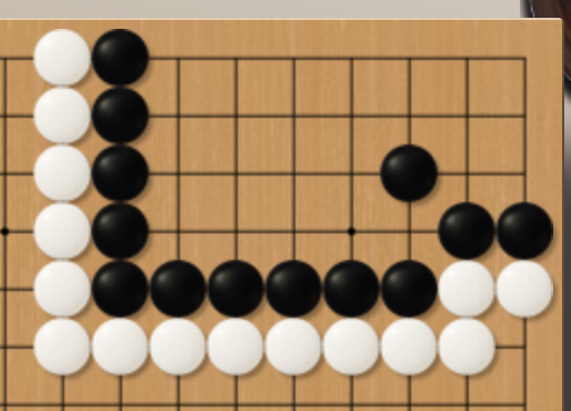
Fig.16 Survival
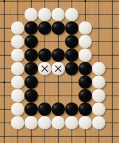
Fig.17 Ancient Chinese Rule and Japanese Rule
Prohibition of the Same Grid Coloring
There is another considerably interesting stalemate in the game of Go. Such a situation is called “Jie” in Chinese while “Ko” in Japanese. The meaning is “aeon”, which originates from a Buddhism concept and describes a very long period. As the literal meaning, the black and white players take the piece from the opponent in turn (see Fig.18). Two sides can be at a stalemate for this single territory from the beginning of the year to Christmas if they repeat this loop. Thus, most rules except the Tromp-Taylor rule prohibit the same grid coloring. If one player attempts to continue to battle for this territory, some move at a different position should be made first. Usually, players will place the piece at a position that threatens the opponent to force the opponent to follow up. If the opponent considers your move at the other area as no threat, the pieces in the “Ko” will be connected by your opponent.
Additionally, there are also some very rare situations with the loop of more than three “Ko”s (See Fig.19).
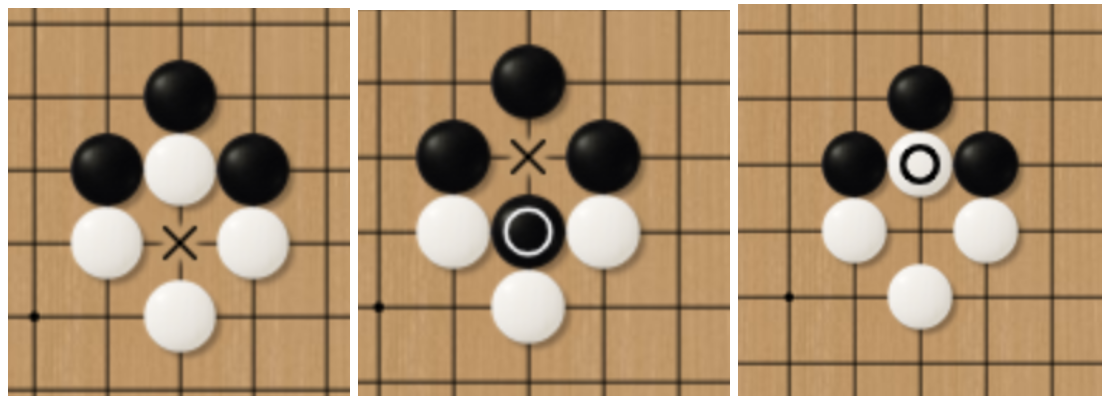
Fig.18 Same Grid Coloring
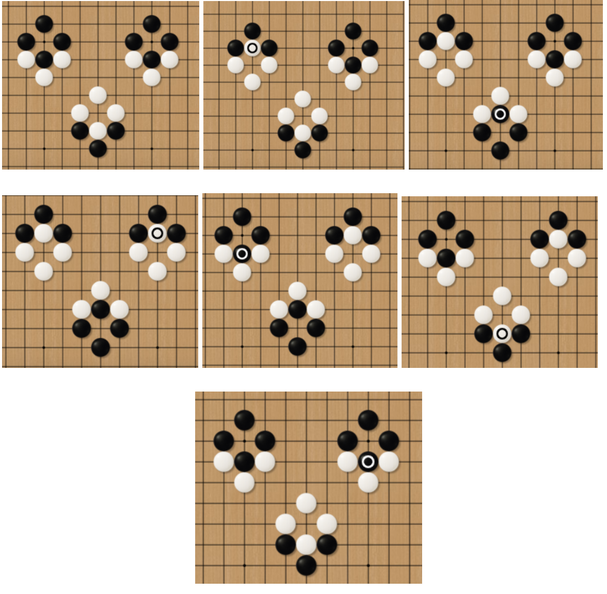
Fig.19 A Loop of Three “Ko”s
Compensation
According to the rule of Go, the black player moves first except the game with a handicap (A players with much higher levels will let the opponent place several pieces at the game board). Thus, the black player is considered as the side with superiority. For the fair play, the black player has to get several points more than the white player for the purpose of winning a game. The number of compensated points are usually 6.5, 7 or 7.5 according to the selected rule. In detail, both the compensation of 6.5 and 7.5 stand for no tie while compensation of an integer allows the tie [3].
Summary
In terms of this project, the rules can be briefly summarized as follows:- The maximum number of moves is set as 722.
- No prohibition of the same grid coloring.
- Count both the surviving pieces and the territory owned by them.
- No double points for the opponent in terms of the taken or dead pieces.
- The compensated points are set as 7.5.
- The game ends after both sides choose the pass.
Project Specification and Methodology
This section illustrates the detailed methodology and analyses the corresponding results of this final design project.
Core Algorithms
The core algorithm employed in this project consists of three important components, including the Monte Carlo tree search, reinforce learning, and convolutional neural network (residual network).
Monte Carlo Tree Search
The Monte Carlo tree search (MCTS) is a classic algorithm, which has been previously leveraged by the famous chess AI “Deepblue”. The primary purpose of this algorithm is to broaden the horizons of the AI player in the aspect of search depth. In other words, the MCTS algorithm gifts AI the ability to predict the future. In detail, the MCTS used for the “Deepblue” adopted the strategy of random guess to search an extremely broad area within a short time. Differently, the AlphaGo Zero utilized the results of the neural network to determine the search direction [1]. In this project, the search strategy is based on the theory mentioned in the AlphaGo Zero but implemented with the simplified details and the reduced tree size. Additionally, the algorithm was programmed in the C programming language and compiled as Python APIs for high-performance computing.
Search Strategy
The search strategy employed in these projects starts searches from the current tree node (current pieces distribution on the board). Each search will end when the search pointer reaches a node that has not been visited or at which the game ends. After one search, the pointer will back up (return) to the original node and update the win rate along the search path. Each move will be determined after 128 searches. The details of each search will be discussed below:
- Forward Search
- Node Extension and Evaluation
- Back Up
- Make a Move
As is shown in Fig.20, the “Q” stands for an action-value (win rate for the black player), which is evaluated by a value network. The “U” stands for the upper confidence bound, determined by the probability distribution for the next step (provided by the policy network) and the visit count stored in the edge between two nodes [1]. Additionally, the larger visit count will result in a lower priority in order to search in different paths. The search priorities in this project are calculated according to the formula below:
For turns of the black player,
Priority = C * Q + T * Prob * sqrt (n{total}) / n{visit}
For turns of the white player,
Priority = C * (1 - Q) + T * Prob * sqrt (n{total}) / n{visit}
where C is a coefficient, T is a temperature coefficient varied according to the search depth, ntotal stands for total visit counts stored in the parent node.
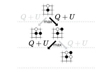
Fig.20 Forward Search [1]
When the search pointer reaches a node that has not been visited, the forward search will end after extending a node [1]. The newly extended node will be evaluated by the outputs from the neural network and corresponding results will be stored.
After extending a node, the search pointer starts to back up (return) to the original node. In detail, the win rate, previously evaluated by the value network, will be updated according to the worst situation (In other words, the optimum move for the opponent). For example, a parent node (black) has three child nodes (white), whose win rates are respectively 40%, 50%, and 60% (The value network always evaluates the win rate for the black player). As a result, the win rate information in the parent node will be updated with a minimum 40% instead of an average of 50%. This classic search strategy in MCTS is called “minimum / maximum search” [5]. Whether to select the minimum or the maximum value is determined by the current player to move. That is because the network only calculates the win rate for the black player. If it is currently the turn for the black player to move, the parent node (white) will be updated with the maximum value.
After repeating the above procedures for 128 times, the MCTS algorithm will make the final decision for the next move, the corresponding formula used in this project are shown below:
For turns of the black player,
Priority = (Qupdated + 0.5) * Prob
For turns of the white player,
Priority = (1.5 - Qupdated) * Prob
Programming Details
As is mentioned above, the MCTS algorithm was programmed in C and compile as Python APIs using Cython (not CPython), which is a Python library working as a bridge between the C and Python. The trees nodes (see Fig.21) store basic information of the current move, the pointer to the parent node, the pointer to the board record, and the pointer to the first edge in the array of the edge struct. Each edge in the edge array, which connects two nodes in the tree, stores the probability distribution of the prediction of the next move, a pointer to the next tree node, and other basic information, such as the visit count.
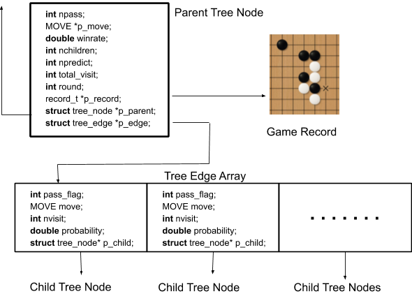
Fig. 21 Structure of the Search Tree
In terms of the virtual loss for the multiple threads, this is a method mentioned in the paper of AlphaGo Zero to add an extremely influential coefficient for the visit count to force each thread search to search in the different paths. In theory, the virtual loss results in huge benefits when the number of cores is large. For example, one TPU has 8 cores. That is because multiple threads search in the same tree and the memory occupation will be sharply decreased (compared with simply starting several threads for generating the data from different games). However, if the search tree is downsized, the probability for two threads to visit the same critical section will substantially increase. The phenomenon of wasting time waiting for the lock will become serious. Furthermore, the locks themselves also occupy the resource and each node needs a lock. Taking all the above factors into consideration, the method of virtual was replaced with simply starting several processes for different games during the training process. Nonetheless, the disadvantages are also obvious. Firstly, the memory occupation will increase with the increase in the number of started threads. Secondly, this method cannot be applied to the user interface because only one game needs to be analyzed.Additionally, the APIs completed in the C are listed as follows:
void call_Pyfunc(PyObject *func, int x[19][19], int y,predict_t *p_predict)
PyObject *import_name(const char *modname, const char *symbol)
void* ego_malloc(int size)
node_repo_t *node_repo_init(void)
node_t* node_repo_add(node_repo_t* sp)
edge_repo_t *edge_repo_init(void)
edge_t* edge_repo_add(edge_repo_t* sp)
record_repo_t *record_repo_init(void)
record_t* record_repo_add(record_repo_t* sp)
void repo_init(repo_t* p_repo)
void repo_free(repo_t* p_repo)
estack_t *stack_init(int size)
int is_empty_stack(estack_t* sp)
int stack_push(estack_t* sp,node_t* p_node)
int stack_pop(estack_t* sp, node_t** p_node)
void stack_free(estack_t *sp)
void predict_game(record_t *p_record, predict_t* result)
void edge_init(predict_t *p_predict,edge_t *p_edge)
void update_record(record_t *p_origin, MOVE *move, int round, record_t *p_next)
double priority_cal(double p, int nvisit, int n_total_visit, int d)
int max_priority(node_t *p_search, double c, int depth)
node_t *node_init(repo_t* p_repo)
node_t *node_create(node_t *p_parent, int select, repo_t* p_repo)
node_t *mcts_init(repo_t* p_repo)
void mcts_search(node_t *p_search, estack_t* p_stack, repo_t* p_repo,int c)
void mcts_backup(estack_t* p_stack)
node_t *mcts_move(node_t* p_head, int n_search, repo_t *p_repo, int c)
int win(record_t* p_game)
void mcts(int n_search, int c)
Experienced Issues
The algorithm of MCTS is a variety of the multi-branch tree. Although the algorithm was not hard to implement, some issues were experienced when the C code was tried to be merged with Python. The first issue we encountered was that the “Python.h” file cannot be found by the C compiler. In the implementation of MCTS, the C code will call python APIs, such as the modules to predict the probability distribution of the next move and win rate. This issue was solved by adding the correct flags and path during the process of compiling. Another issue was that the grammar of Cython is a little different from C. For example, there is no “->” in Cython. Instead, anything pointed by a pointer of a struct should be linked with “.” in Cython. Furthermore, although the algorithm was implemented according to the paper of AlphaGo Zero, the DeepMind team omitted a lot of significant details, such as the some critical parameters. To improve the performance, it took a lot of time to adjust the details of the algorithm.
Testing
The algorithm of MCTS was programmed in a highly modularized way. Thus, the testing was performed by unit. Thus, the unit test was performed for each module to make sure that the API provided the expected functions.
Convolutional Neural Network
The conventional convolutional neural network (CNN) always face an adverse situation that the gradient explodes or disappears when the number of layers increases. As a classic solution, the residual network (ResNet) creatively constructs the residual blocks, which remains the block input (see Fig.22) [6]. In other words, the ResNet blocks are trained based on the difference between the block inputs and outputs. As a result, the ResNet results in a much deeper CNN (with more layers).
According to the research on the best inputs and outputs for the network, the pure piece distribution (19x19) is considered to have optimum performance [1] [7]. Additionally, the previous networks (before AlphaGo Zero) also utilized a lot of human knowledge, such as liberty. Furthermore, the AlphaGo Zero combined the policy network and the value network to make them share the same “body” [1].
In this project, the convolutional neural network was constructed based on the theory of ResNet using TensorFlow 2.0. The structures for residual units and residual blocks, which consist of several residual units, are shown in Fig.22 and Table.1. In detail, each residual unit consists of three convolutional layers, whose sizes of the convolution kernel are respectively 1x1, 3x3, 1x1. Moreover, the batch normalization layer and activation layer are placed before the convolution layers [6] (different from the conventional designs). Last but not least, the network has two inputs and two outputs, which share the same body (see Fig.23). The neural network was trained as a classifier (The outputs of a classifier are actually probability distribution and the outputs activated by the softmax will have the sum of 1). Additionally, the strategy of L2 regularization was employed to restrain the overfitting.

Fig.22 Structure of the Residual Unit Constructed in this Project

Fig.23 Combination of the Policy Network and the Value Network
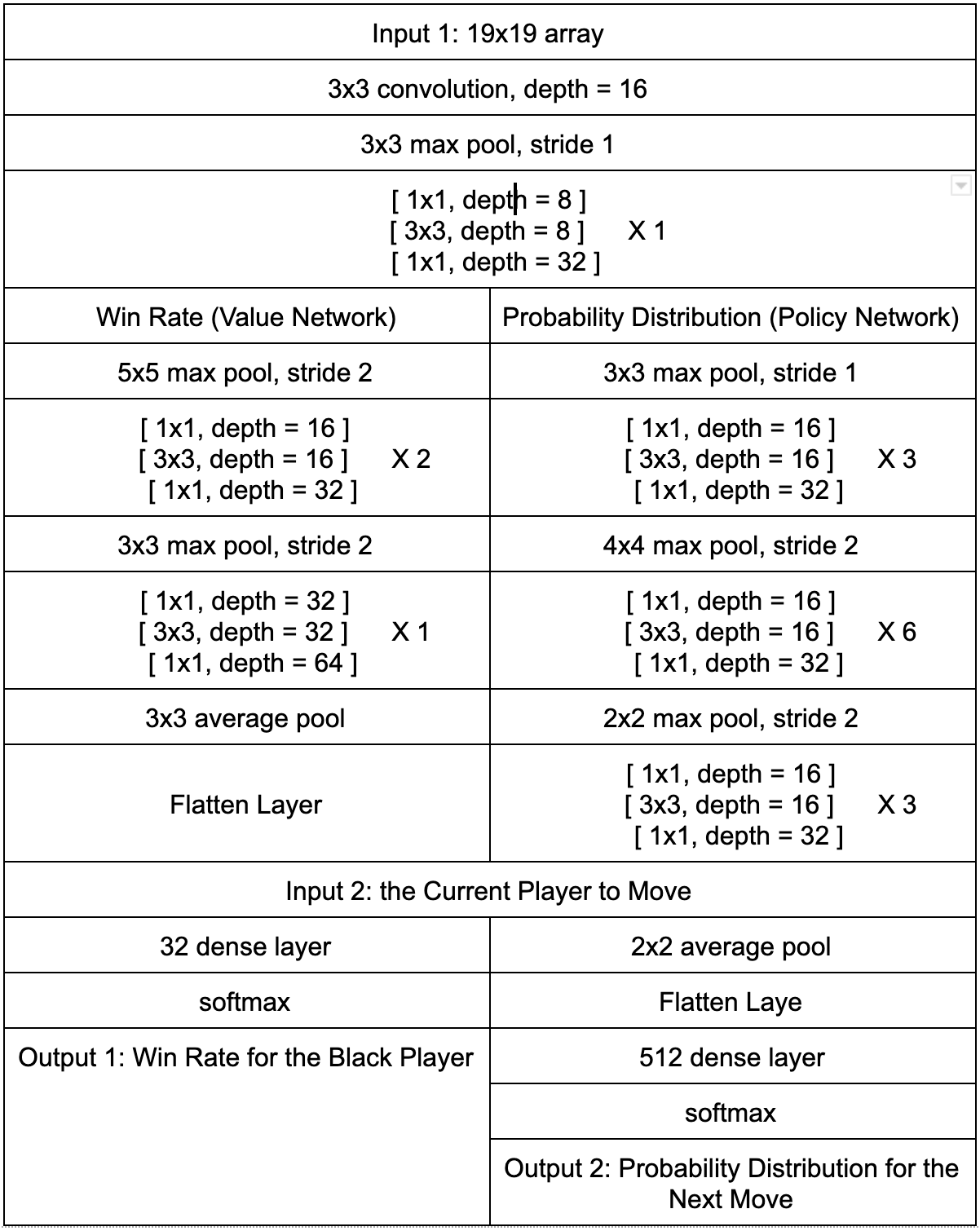
Table 1. The Structure of the Residual Network
Experienced Issues
An encountered issue was that the training of the network was found slowed down after the long time running. Obviously, this is usually caused by bad memory utilization. After checking and testing the details in the code, it was finally found that a new model will be created (loaded from the lastly save checkpoints) after a dataset was finished. However, the previously loaded model was not deleted (It can still be called in the experiments). Thus, the solution was to delete the previous model before reloading. Finally, this issue was effectively relieved.
Testing
The efficiency and effectiveness of the ResNet was tested on the dataset “cifar10”, which is a triple-channel (colored) 32x32 image sets (see Fig.24). The accuracy was compared with the tutorial published by Google [8]. In terms of the unreinforced datasets, the accuracy of the ResNet (not very deep in this test) is 81%. Compared with the traditional CNN model provided by Google in the tutorial, whose accuracy is 70%, the ResNet performed much better. After reinforcing the datasets, the accuracy of the ResNet and traditional CNN model finally reached 92% and 79% respectively. The performance of the neural network for the Go AI is actually hard to evaluate. Hence, a relative evaluable dataset was tested first to make sure that the project moved forward on the right way.
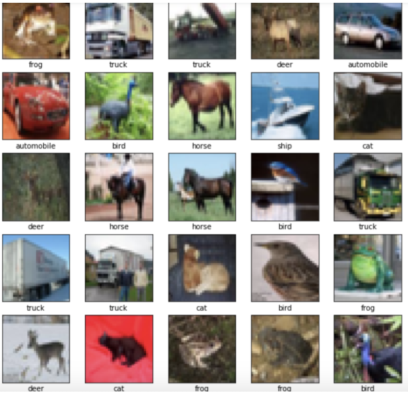
Fig. 24 Cifar10 Dataset
Reinforcement Learning
Reinforcement learning is realized based on the above two algorithms. In order to judge whether some pieces will be taken after each move, an extra API is implemented using the deep-first search (DFS) algorithm. In detail, the pointer starts searching from the position to move. All of the four neighbors will be searched. Taking Fig.25 as an example, the position to move (the turn of white) is marked with the star. The pointer searches all four neighbors. The pointer will keep search until finding the liberty of black pieces or traverses all connected black pieces. If an unsearched black piece is found, it will be pushed into a stack. Moreover, a 19x19 array is employed to record the visited positions in order to avoid repeated searches. The method to judge suicide is the same as mentioned above (also the DFS algorithm). Furthermore, in terms of evaluating the winner, the dead pieces will be removed from the game board first (also the DFS algorithm). Then the territory will be traversed with the DFS algorithm again. The only difference is that the pointer searches for the pieces with liberty previously while in this situation the pointer searches for the territory surrounded by pieces. Additionally, the intermediate zone, which never happens in human games, will be equally divided to both players (see Fig.26).
With respect to the rewards of reinforcement learning, each move in the game will be extracted as a training sample. As has been mentioned above, the outputs of a classifier are actually probability distribution. Thus, all the samples in the same game with be labeled with the game result (Black wins: 0, White wins: 1). Similarly, for the loser, the prediction on the adjusted next move will be randomly selected according to the corresponding probability distribution (The moves of the loser will not be selected).
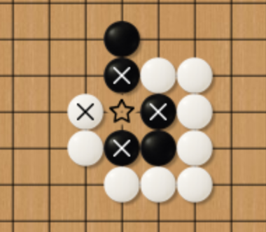
Fig.25 Deep-first Search
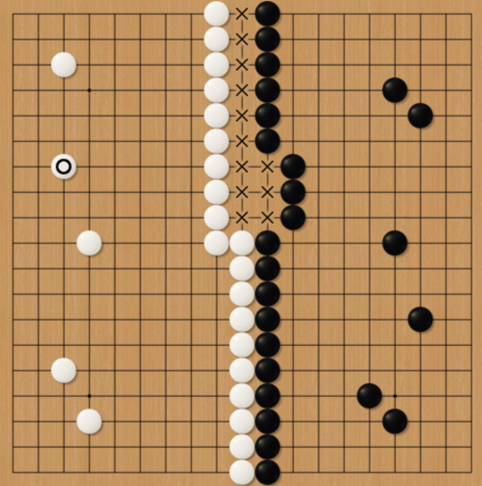
Fig.26 Intermediate Zone
Experienced Issues
The modules of reinforce learning and MCTS were connected with the Residual Network in the pattern of producer and consumer. An issue was encountered when the consumer tried to check whether the folder is empty. The consumer was detected to keep loading the model and reading from the folder when the folder is empty. The issue was finally solved by excluding the path of the “.DS_Store” file, which is an invisible file generated by the “finder”.
Testing
The algorithm of reinforce learning was partly embedded in modules of the MCTS algorithm. Thus, the testing of reinforce learning was performed similar to the that of MCTS (by unit).
User Interface Design and Implementation
Framework and Brief Description of Data structure
The implementation of the user interface (UI) was constructed based on Pygame, which is a cross-platform integration of Python modules. According to the experience accumulated in the previous labs, the Pygame was anticipated to show stable performance.
This section will state some data structures used in the UI for the purpose of a clear explanation of the entire work. The entire UI is divided into two parts. The first part is logic and computation and the second part is for displaying all elements on the board. Comparing to the core algorithm, the UI implementation of data storage and other logic of the Go rules are quite different. Taking the hardware of the Raspberry Pi into consideration, it is too weak to store huge data and execute complex computation work. For example, there are 19 * 19 = 361 crossing points located on the board, storing everything in a 2D matrix is much easier and convenient for following tree search, however, for Pygame re-rendering which is a frequent job, it takes approximately one second to traverse all the points. It’s unacceptable for user experience. For another instance, taking pieces is really intuitive for humans, however, the computer needs to search every possible position multiple times to finish taking pieces. For UI, we use the union-find algorithm to fulfill the function however in the search process, we design a regular DFS process for searching because compared to the search process, DFS takes much less resource and too much logic code complicates the logic of search.
- Store pieces on the board: 2D array for storing only those points which have been occupied by the pieces.
- Union-find algorithm: A list is used for storing the parent node for each group.
- Mouse coordinates: A list containing only 2 points
- Turn: White or black?
Background Board Draw
From the initial thought, we tried to find a board image with fitting-well size for the board. However, we got no rewards for our hard search. Displaying background of the wood-like texture is the whole job for the image. The grid of the board is all drawn by the python with multiple benefits:
- It is easy to place a precise position for every single piece. Every line shown on the board is drawn by the codes we wrote. For example, we know what is the exact width in pixel from the outline to the board border.
- For further functions such as removing the piece, re-rendering board and even moving the mouse, a grid made by us empowers more flexibility. Each function will be discussed in detail in the below sections.
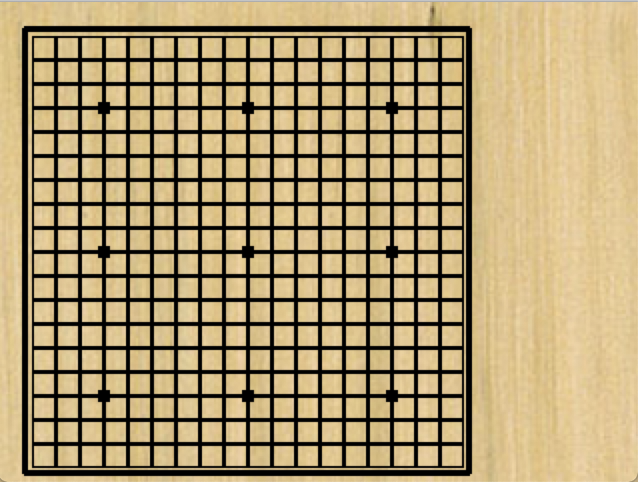
Fig.27 Go Board Background
Mouse Design
Initially, we designed that using the touch screen to place the piece but a high rate of mistake touch due to small screen size leading us to redesign the interactive mechanism. The other back-up plan is simulating a mouse displaying on the board. The go game offers 6 physical buttons for up (GPIO.17), down (GPIO.22), left (GPIO.23), right (GPIO.27), place (GPIO.19) and exit (GPIO.26). The move of the mouse is located on the exact crossing point of the grid. When the player clicks the place button, the piece will be placed.
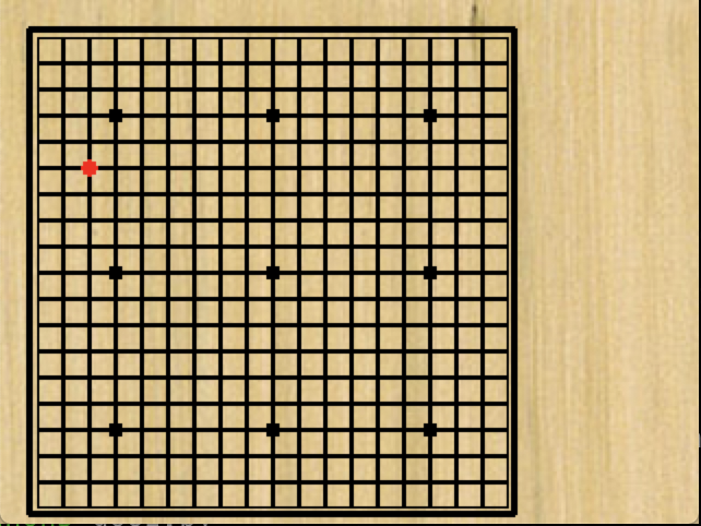
Fig.28 Mouse Design
Draw Pieces
A piece essentially is a 6-pixel black circle. When the user clicks the place button, Pygame will draw the piece on the position according to the mouse position. UI passes the current coordinate to the back-end logic for storing, judgment and update.
Remove Pieces
When it comes to removing a piece, it’s a totally different story. If the back-end tells the UI that some pieces should be removed after current placement, Pygame should re-render the UI. Considering of massive data and resource cost (For Raspi), it is impossible to draw everything again even if most of them are still in the same shape.
We came up with a feasible solution: A to-be-removed piece first covered by a Pygame rect, and the rest of the work is to re-draw that crossing point area. It is not too tough due to knowing the whole layout of the board.
High-Efficiency Algorithm for Removing Piece
As mentioned above, the removing algorithm is implemented using DFS, which is a naive algorithm. Although the program does not store any other information saving some space, it has high time complexity. Hence, we adopt union-find to decrease the time complexity. We define a group as an area containing all connected pieces in the same color. All pieces in the same group have the same parent piece, which is chosen randomly. The visualization of the group looks like a tree, the root node is the parent. When two groups merge, the program prefers to merge the tree with a lower height to the tree with a higher height. That is, the rank of the tree is minimum so that optimize the update time.
Predict Best Nine Hands
You may notice that there is an empty area on the right side of the board. It is used for displaying the best nine hands for the current turn. For example, if the current turn is white, the list shows the best nine hands for white. The list is sorted by the win rate, and the possibilities of each step are given. The possibility is the chance of choice for the next step from pro players.
Evaluation
Model Accuracy Evaluation
After the training of four days with optimized parameters, which were experimented using downsized models, the final CNN model reached an accuracy of 18% and 78% on the testing datasets for the outputs of prediction on next move and winner respectively. The testing dataset was compared with data from the human professional players (with a level higher than the professional 4 dan). As a contrast, the European Go champion, who was the first famous player defeated by the AlphaGo, possesses a level of professional 2 dan [9]. An accuracy of 18% for the prediction on the next move seems quite a low value. Nonetheless, the game of Go is a considerably complicated abstract strategy game. Moreover, in terms of each move, there is possible more than one good positions to move. Thus, the accuracy on the next move will not reach a high level, even though the testing data are collected from the game record of the human professional players. In addition, the accuracies of AlphaGo Master and AlphaGo Zero are respectively 60% and 50% (The better model even has a relatively lower accuracy on the human dataset, although it definitely does not mean an accuracy of 18% is better than 50%). Furthermore, an accuracy of 18% stands for the model can accurately predict a professional player every 5 moves. The remaining 4 predictions can still be good positions (or not bad) to move because good moves are usually unique. Conclusively, the accuracy of 18% is an acceptable value for a lightweight ResNet (with 6 residual blocks and total 55 layers).
In terms of the weakness of this model, even the MCTS algorithm was employed, the entire model sometimes shows bad performance on the evaluation for a large number of connected pieces (a term of Go to describe such pieces: dragon). This kind of connected pieces usually distribute across the whole game board but have difficulty making two true eyes (In other words, surviving). The size limitation of the convolutional kernel makes the model sometimes hard to recognize the “dragon” (a large number of connected pieces) even with the help of the MCTS algorithm. That is because the MCTS provides a foothold to “observe” the future instead of the whole game board. In other words, the MCTS algorithm works on the aspect of depth instead of width. Hence, a feasible solution, which has been applied to this project, is to construct a parallel network, whose input nodes and output nodes are connected to the original network, with larger sizes of convolution kernels. The original network will be used to analyse the local information while the other one owns the global sight.
System Performance
In this section, we discuss the impact of the program on the Raspi. All data below is the mean value.
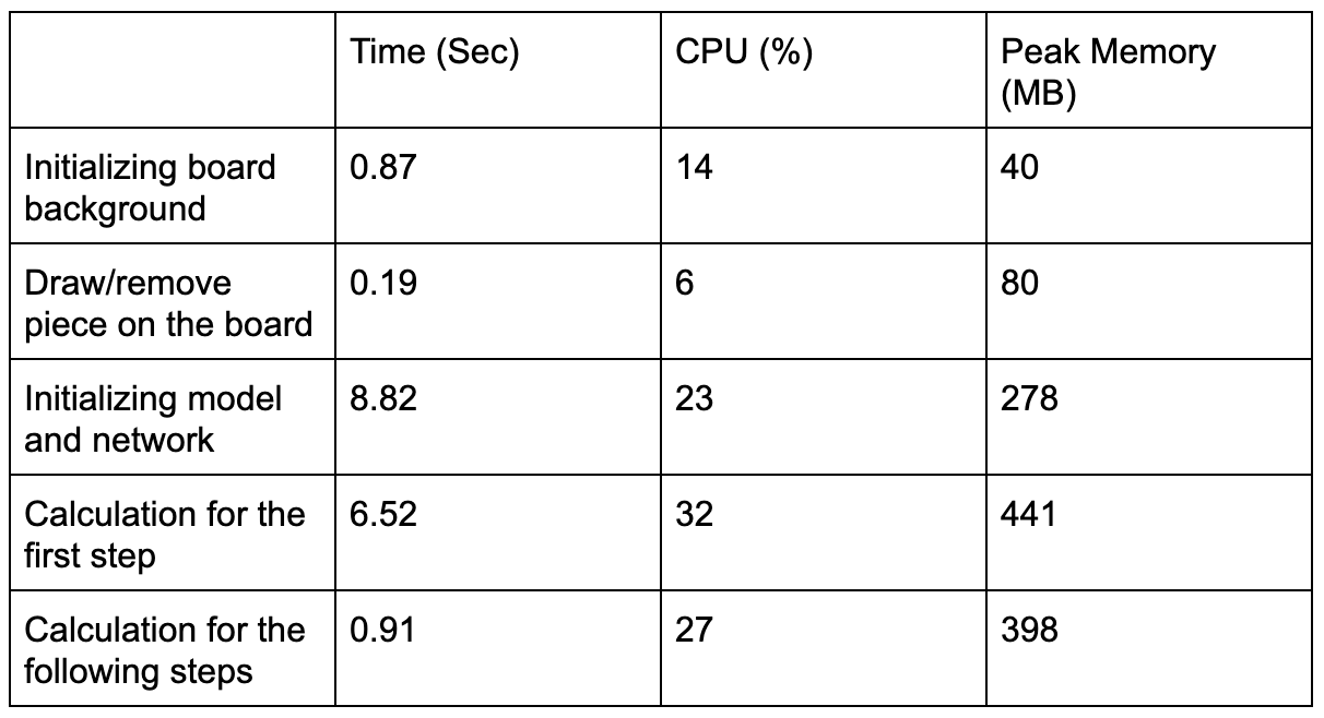
Table 2. System Performance Evaluation
When it comes to the search algorithm, we optimized it to utilize multiple cores of the processor.
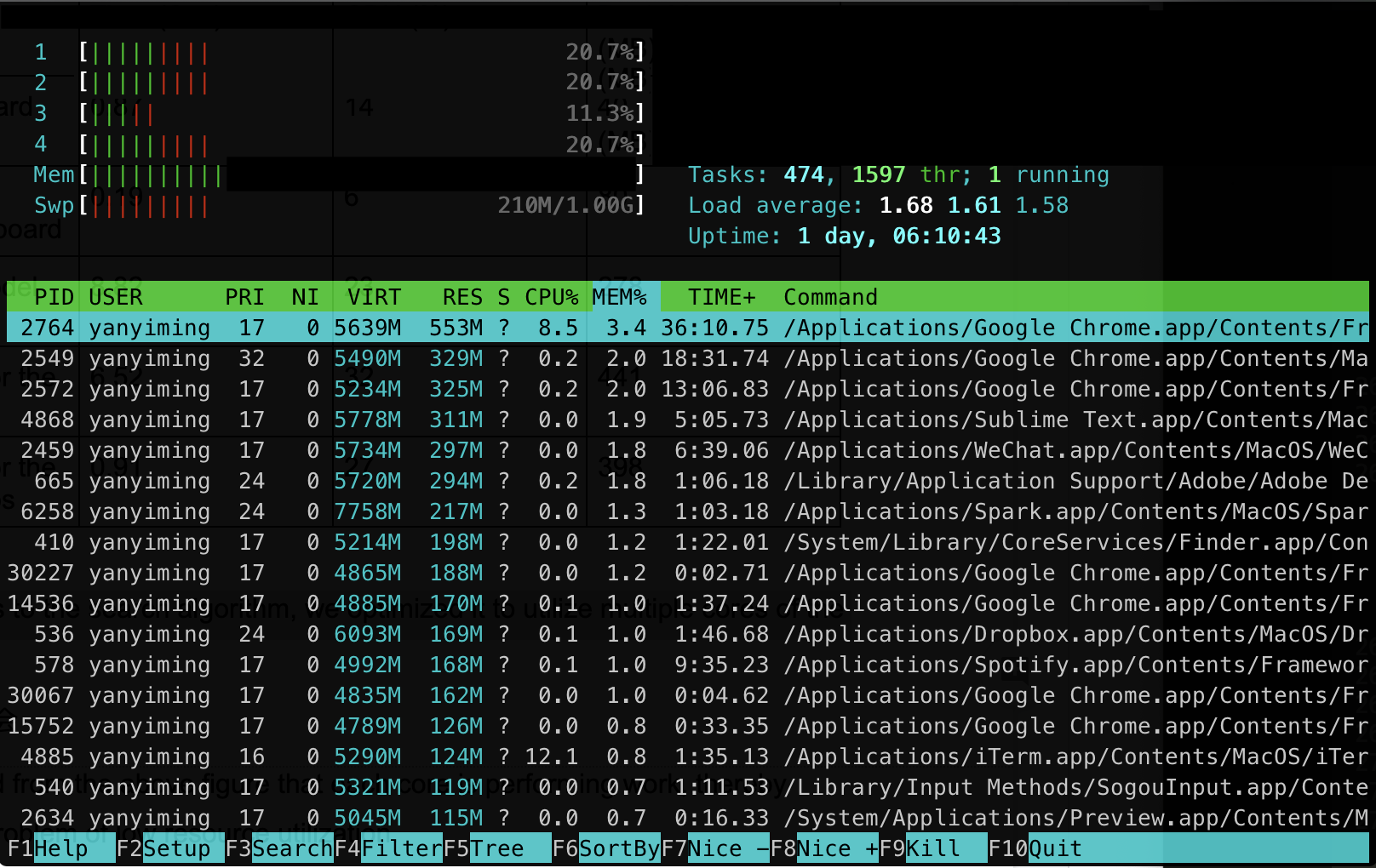
Fig.29 Htop for Searching
It can be found from the above figure that each core is performing work, thereby avoiding the problem of low resource utilization.
Result
The entire project plan was generally smooth. The majority of the encountered issues have been discussed in the previous sections.
In terms of the initial goal, the main goals have been completed. In detail, some adjustment was made according to the corresponding research and actual conditions. With respect to the core, the original plan was to use human data to train the neural network while the method reinforce learning was finally employed (It is believed that reinforce learning performs better than pure human datasets). In regards to the UI, the original plan of placing pieces with touch was replaced with the plan of placing pieces with buttons. That is because the touch may result in results different from the users’ expectations.
Conclusion
We finally completed an intelligent Go game analyzer with powerful performance within a relatively tight time frame. Not only can it implement all the rules of Go, but it can also provide the predictions on the best next moves for the players on both sides. In terms of the original plan, the touch screen was planned to be used to control the entire chessboard, but through experience testing, we found that this design is entirely unfeasible. The first is that designing too many touch areas on a smaller screen can increase false touches. Another disadvantage is that too many touch areas increase the resource consumption required by the program due to event judgment, which results in the program running slowly and far from meeting our expected speed. In terms of further improvement, a feasible idea is to combine the touch screen and buttons. The players generally touch first and adjust their moves with buttons.
Future Wowk
In the current phase, both the core algorithm and user interface are completed and functional. In terms of the future work on the core algorithm, the current MCTS algorithm has poor support for the full utilization of thread advantage on the four cores of the Raspberry in terms of the user interface (The design only took the training process into consideration. That is actually a mistake in terms of this viewpoint). In future work, the method of virtual loss, which mentioned in the previous sections, will be employed to improve the performance of the MCTS in the environment of the user interface. With respect to the future work on the user interface, first, the current piTFT with a relatively small size can be replaced with a larger touch screen for better user experience. There will be a lot of changes in the code for drawing, which mainly involve the reconstruction on the pixel level. Last but not least, the predictions for the next move can be marked on the screen from 1 to 9 with numbers according to the priority. Additionally, the APIs with the functions of predicting the win rate of the current move and evaluating the winner, which have been realized in the core algorithm and applied to the training of the model, have not been connected to the front-end. This is also remaining work for the future.
Budget
In regard to the actual training, the process was completed (lasting four days) on a borrowed high-performance computer, equipment with the AMD Ryzen 7 3800X processor and the RTX 2080 Ti graphics card. Before the formal training, a set of controlled experiments (with downsized models) were previously implemented on the laptop in order to optimize the parameters. Although the training device was provided for free, the cost can still be converted in accordance with the AWS device with similar performance ($0.7 / hour). Thus, the total cost of computation was approximately $67.2.
Work Distribution

Yiming Yan | Peihan Gao
yy852@cornell.edu | pg477@cornell.edu
User Interface Design | Search Algorithm Design
References
[1] DeepMind, “Master the Game of Go without Human Knowledge”, https://www.nature.com/articles/nature24270.epdf?author_access_token=VJXbVjaSHxFoctQQ4p2k4tRgN0jAjWel9jnR3ZoTv0PVW4gB86EEpGqTRDtpIz-2rmo8-KG06gqVobU5NSCFeHILHcVFUeMsbvwS-lxjqQGg98faovwjxeTUgZAUMnRQ, 2017.[2] J. Tromp, “The game of Go, aka Weiqi in Chinese, Baduk in Korean”, http://tromp.github.io/go.html.
[3] World Mind Sports Games 2008, “Rules of Go (Weiqi)”, http://home.snafu.de/jasiek/WMSGrules.pdf, Jul, 2008.
[4] The International Go Federation, “Go Population Survey”, http://www.intergofed.org/wp-content/uploads/2016/06/2016_Go_population_report.pdf, Feb, 2016.
[5] G.M.J.B. Chaslot, M.H.M. Winands, J.W.H.M. Uiterwijk, H.J. van den Herik, B. Bouzy, "Progressive Strategies for Monte-Carlo Tree Search", https://dke.maastrichtuniversity.nl/m.winands/documents/pMCTS.pdf, 2008.
[6] K. He, X. Zhang, S. Ren, J. Sun, “Deep Residual Learning for Image Recognition”, https://www.cv-foundation.org/openaccess/content_cvpr_2016/papers/ He_Deep_Residual_Learning_CVPR_2016_paper.pdf, 2016.
[7] C. Clark, A. Storkey, “Training Deep Convolutional Neural Networks to Play Go”, http://proceedings.mlr.press/v37/clark15.pdf, 2015.
[8] Google, “Convolutional Neural Network (CNN)”, https://www.tensorflow.org/ tutorials/images/cnn, 2019.
[9] DeepMind, “AlphaGo”, https://deepmind.com/research/case-studies/alphago-the-story-so-far, 2019